ibei - Calculator for incomplete Bose-Einstein integral

The Bose-Einstein integral appears when calculating quantities pertaining to photons. It is used to derive the Stefan-Boltzmann law, and it also appears when calculating the detailed balance limit of a solar cell as described by Shockley and Queisser [SQ61] , and when calculating the photo-enhanced thermoelectron emission from a material as described by Schwede et.al. [SBR+10] .

The ibei module provides functionality to calculate various forms of the Bose-Einstein integral, along with well-known models of photovoltaic devices. The ibei module provides a ibei.BEI class which includes methods to compute the full, upper-incomplete, and lower-incomplete Bose-Einstein integrals. It also includes two convenience classes for calculating the power density and efficiency of a single-junction solar cell according to Shockley and Queisser [SQ61] and deVos [deV92]. See the Mathematical Description and Applications section for the mathematical details.

Installation

This package is installable via pip.

pip install ibei

Alternatively, download the source, install hatch, and build.

git clone git@github.com:jrsmith3/ibei.git
pip install hatch
hatch build
pip install dist/ibei-1.0.6.tar.gz  # Or whatever is the latest version in that directory.

Examples

Calculate the number of above-bandgap photons from Si at 300K:

>>> import ibei
>>> bandgap = 1.1
>>> bei = ibei.BEI(order=2, energy_bound=bandgap, temperature=300., chemical_potential=0.)
>>> bei.upper()
<Quantity 10549124.09538381 1 / (m2 s)>

Verify Shockley and Queisser’s result [SQ61] that the efficiency of a silicon solar cell is 44%:

>>> import ibei
>>> solarcell = ibei.SQSolarcell(solar_temperature=6000., bandgap=1.1)
>>> solarcell.efficiency()
<Quantity 0.43866807>

Plot efficiency vs. bandgap of a single-junction solar cell as in Shockley and Queisser’s Fig. 3 [SQ61]:

>>> import ibei
>>> import numpy as np
>>> import matplotlib.pyplot as plt

>>> bandgaps = np.linspace(0, 3.25, 100)
>>> efficiencies = []
>>> for bandgap in bandgaps:
...     solarcell = ibei.SQSolarcell(solar_temperature=6000, bandgap=bandgap)
...     efficiency = solarcell.efficiency()
...     efficiencies.append(efficiency)

>>> plt.plot(bandgaps, efficiencies)
>>> plt.xlabel("Bandgap (eV)")
>>> plt.ylabel("Efficiency")
>>> plt.show()

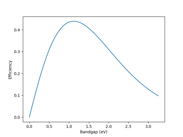
Efficiency vs. bandgap of a photovoltaic using Shockley and Queisser's model. — Efficiency vs. bandgap of a photovoltaic using Shockley and Queisser’s model [SQ61].

API Reference

Base Library (ibei)

Mathematical Description and Applications

The Bose-Einstein integral, subsequently referred to as the “full Bose-Einstein integral” or “full integral”, is denoted \(G_{m} (T, \mu)\) and is given by Eq. (1).

(1)\[G_{m}(T, \mu) = \frac{2 \pi}{h^{3} c^{2}} \int_{0}^{\infty} E^{m} \frac{1}{\exp(\frac{E-\mu}{kT}) - 1} dE\]

The quantity \(h\) is Planck’s constant, \(c\) is the speed of light, \(\mu\) is the chemical potential of photons, \(E\) is the energy of photons, \(T\) is the temperature of the radiator, and \(k\) is Boltzmann’s constant.

Now consider the two integrals \(G_{m} (E_{g}, T, \mu)\) and \(g_{m} (E_{g}, T, \mu)\), called the upper-incomplete Bose-Einstein integral and the lower-incomplete Bose-Einstein integral, respectively, and given by Eqs. (2) and (3), respectively.

(2)\[G_{m} (E_{g}, T, \mu) = \frac{2 \pi}{h^{3} c^{2}} \int_{E_{g}}^{\infty} E^{m} \frac{1}{\exp(\frac{E-\mu}{kT}) - 1} dE\]

(3)\[g_{m} (E_{g}, T, \mu) = \frac{2 \pi}{h^{3} c^{2}} \int_{0}^{E_{g}} E^{m} \frac{1}{\exp(\frac{E-\mu}{kT}) - 1} dE\]

The two integrals given above can be summed to form a relationship between the full, upper-incomplete, and lower-incomplete Bose-Einstein integrals.

(4)\[G_{m} (T, \mu) = G_{m} (E_{g}, T, \mu) + g_{m} (E_{g}, T, \mu)\]

The integration of the full Bose-Einstein integral can be performed to yield the expression given in Eq. (5).

(5)\[G_{m}(T, \mu) = \frac{2 \pi (kT)^{m+1}}{h^{3} c^{2}} \Gamma(m+1) Li_{m+1}\left(\exp\left(\frac{\mu}{kT}\right)\right)\]

where \(\Gamma(z)\) is the gamma function and \(Li_{s}(z)\) is the polylogarithm of index \(s\). The upper-incomplete Bose-Einstein integral can be expressed as a finite sum of polylogarithm functions as shown by Smith (reference forthcoming) and given in Eq. (6).

(6)\[G_{m}(E_{g},T,\mu) = \frac{2\pi m! (kT)^{m+1}}{h^{3} c^{2}} \sum_{s = 1}^{m+1} \frac{1}{(m-s+1)!} \left( \frac{E_{g}}{kT} \right)^{m-s+1} Li_{s} \left( \exp \left( \frac{\mu - E_{g}}{kT} \right) \right)\]

An expression for the lower-incomplete Bose-Einstein integral can be obtained by solving Eq. (4) for \(g_{m} (E_{g}, T, \mu)\) and substituting Eqs. (5) and (6) for the full and upper-incomplete integrals, respectively.

License

The code is licensed under the MIT license. You can use this code in your project without telling me, but it would be great to hear about who’s using the code. You can reach me at joshua.r.smith@gmail.com.

Contributing

The repository is hosted on github . Feel free to fork this project and/or submit a pull request. Please notify me of any issues using the issue tracker .

In the unlikely event that a community forms around this project, please adhere to the Python Community code of conduct.

Developer Notes

This section contains information about some common tasks that are needed during the course of development. I restarted work on this repo years after I last worked on it, so I’m mainly writing these notes to my future self if that situation happens again.

This repository uses tox (link) for most of its automation, so install it before hacking on the source.

# Install dependencies for development.
pip install tox

To run the tests, just call tox. tox will install the necessary dependencies (e.g. pytest) in a virtual environment, build the package, install the package that was built (which is a good practice) into that virtual environment, then call pytest to run the tests.

# Run the tests in your local environment.
tox

This repo uses sphinx to create this documentation. There is a tox environment definition to build the documentation; the documentation can be built locally as follows.

# Build the documentation in your local environment.
tox -e doc

This approach provides all the same advantages as using tox for testing, namely, the only dependency that must be installed on the local system is tox, and tox itself manages all of the other dependencies in a virtual environment.

Invocations of tox will add some files to the local filesystem, and there is a small risk that these files accidentally get committed to the repo. Use the following command at the root of the repo to clean up.

# Clean up build artifacts.
git clean -fx .

This repo also features GitHub workflows for continuous integration automations. Some of these automations leverage tox as well, and there are corresponding tox environments defined in the tox.ini file. These tox environments are not intended to be run on a developer’s machine – see the tox config and the automation definitions in the .github subdirectory for information on how they work.

Version numbers are PEP 440 compliant. Versions are indicated by a tagged commit in the repo (i.e. a “version tag”). Version tags are formatted as a “version string”; version strings include a literal “v” prefix followed by a string that can be parsed according to PEP 440. For example: v2.0.0 and not simply 2.0.0. Such version strings will have three components, MAJOR.MINOR.PATCH, which follow clauses 1-8 of the semver 2.0.0 specification. Any documentation change by itself will result in an increment of the PATCH component of the version string.

All commits to the main branch will be tagged releases. There is no dev branch in this repo. This repo will likely not include prerelease versions. This repo may include post-release versions. Such post-release versions correspond to changes to the development infrastructure and not functional changes to the codebase. Such post-release versions may result in a new build posted to PyPI, but it would be good if they didn’t.

This repo includes a GitHub workflow to automatically build the package, test the package, create a GitHub release, and upload the package to PyPI when a version tag is pushed. Version tags are manually created by me (Joshua Ryan Smith) in my local clone of the repo. Therefore, releasing is semi-automated but is initiated by a manual tagging process. I.e. when I want to create a new release, I create a version tag in the repo and push that tag – the GitHub workflows take care of the rest. Such version tags should be annotated. The tag message should include the list of issues that are included in the release.

Citing

You can cite this software as follows.

Smith J.R. ibei (version x.y.z). URL: https://ibei.readthedocs.org

The repo contains a CITATION.cff file (content given below) formatted as cff. Tools like cffconvert exist to convert the cff data to other formats, like BibTeX.

cff-version: 1.2.0
title: "ibei"
abstract: "Calculators for Bose-Einstein integrals."
repository-code: "https://github.com/jrsmith3/ibei"
url: "https://ibei.readthedocs.org"
type: software
license:
  - MIT
authors:
  - family-names: Smith
    given-names: Joshua Ryan
    orcid: "https://orcid.org/0000-0002-3137-7180"
contact:
  - family-names: Smith
    given-names: Joshua Ryan
    email: joshua.r.smith@gmail.com
keywords:
  - Bose-Einstein integral
  - Bose-Einstein statistics
  - python
  - thermal radiation
message: "Use information in this file when citing this software."

Bibliography

deV92: Alexis deVos. Endoreversible thermodynamics of solar energy conversion. Oxford University Press, Oxford New York, 1992. ISBN 9780198513926.
SBR+10: Jared W. Schwede, Igor Bargatin, Daniel C. Riley, Brian E. Hardin, Samuel J. Rosenthal, Yun Sun, Felix Schmitt, Piero Pianetta, Roger T. Howe, Zhi-Xun Shen, and Nicholas A. Melosh. Photon-enhanced thermionic emission for solar concentrator systems. Nat Mater, 9(9):762–767, Sep 2010. doi:10.1038/nmat2814.
SQ61(1,2,3,4,5): William Shockley and Hans J. Queisser. Detailed balance limit of efficiency of p‐n junction solar cells. Journal of Applied Physics, 32(3):510–519, 1961. doi:10.1063/1.1736034.